Fundamentals of Retrieval Augmentation Generation (RAG)
Retrieval Augmentation Augmentation (RAG) is an emergent topic which allows the use of your personal/private data with Large Language Models (LLMs).
RAG makes LLMs more powerful by giving them access to external knowledge, which can be your personal documents, Wikipedia, etc. Avoiding the need to fine-tune the LLMs with your own data, which can be expensive and time consuming.
On this post will cover the fundamentals of RAG, which is a combination of Information Retrieval (IR) and Seq2Seq Models and show how the field has been emerging in the last years.
Table of Contents
- Information Retrieval (IR) (1951-1992)
- Representing documents in a Vector Space Model (1975+)
- Numerical words representations have semantics (2013+)
- Generating text with Seq2Seq Models (1980+)
- Synthesizing documents and generated text (2020)
Information Retrieval (IR) (1951 - 1992)
Information Retrieval (IR) is a metholodigy which was presented by Philip Bagley in 1951 at MIT. He presented the idea of a machine that could store, organize and retrieve any type of data (e.g., text, images, audio, etc) efficiently.
Different from SQL queries of a database where you can get the data you want with a match, with IR you can get the most relevant documents based on a query. For example, if you search for What is the capital of Brazil? you will get the most relevant documents based on the query, which can be Brasilia is the capital of Brazil or Brazil is a country in South America`.
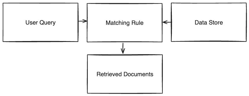
Following the diagram above, we have the following blocks:
1. User Query: The user query is the input of the IR system, which can be a text, image, audio, etc.
2. Matching Rule: The matching rule is responsible to match the user query with the documents in the database.
3. Data Store The data store is the database that stores the documents.
4. Retrieved Documents The retrieved documents are the documents that matched the user query.
These blocks are the fundamentals of IR, and there are different approaches to implement each one of them. For example, the matching rule can be implemented using a Vector Space Model or Probabilistic Model. We will cover the Vector Space Model in the next section.
In 1992 the US Department of Defense conspored Text Retrieval Conference Text Retrieval Conference to encourage research in the field of text retrieval. The first conference was held in 1992 and the last in 2016. Where they provided a infrastructure to test and compare different approaches to text retrieval incentivizing the research in the field.
Representing documents in a Vector Space Model (1975)
The Vector Space Model (VSM) was first introduced in 2013 in the paper A Vector Space Model for Automatic Indexing by Gerard Salton and Michael J. McGill. The VSM is a model that represents documents as vectors in a multidimensional space, where each dimension corresponds to a separate term.
Measuring Document Similarity
Document similarity is a measure of how similar two documents are where we compare the terms of each document and calculate the distance between them. For example, if we have two documents:
doc1 = "Brazil is a country in South America"
doc2 = "Brasilia is the capital of Brazil"
We can represent each document as a vector where each dimension is a term and the value is the frequency of the term in the document. For example, if we have the following terms:
terms = ["Brazil", "South", "America", "Brasilia", "Capital"]We can represent the documents as:
doc1 = [1, 1, 1, 0, 0]
doc2 = [1, 0, 0, 1, 1]
Then we can calculate the similarity between them. Using cosine Similarity or maximum inner product search (MIPS) to find the most similar documents.
similarity = cosine_similarity(doc1, doc2)There are different approaches to calculate the similarity between documents, and each one has its own advantages and disadvantages. For example, cosine similarity is a simple approach to calculate the similarity between documents, and different from MIPS it doesn’t count the frequency of the terms.
Numerical words representations have semantics (2013)
With the advancement of neural networks and natural language processing (NLP), Word2Vec was presented in 2013 by Tomas Mikolov and his team, to solve NLP problems where words are tratated as atomic, isolated units (e.g., “cat” and “dog” are treated as different words, even if they are semantically related).
For this problem, was proposed a new neural network architecture that learns word embeddings from large datasets. Using a neural network to learn the semantics of the words and represent them as vectors. With this approach we can calculate the similarity between words and documents. Below the two approaches to train the Word2Vec model:
Continuous Bag-of-Words (CBOW)
The CBOW model predicts the current word based on the context. For example if we have the sentence “The cat is on the mat”, the model will predict the word “cat” based on the context “The __ is on the mat”.
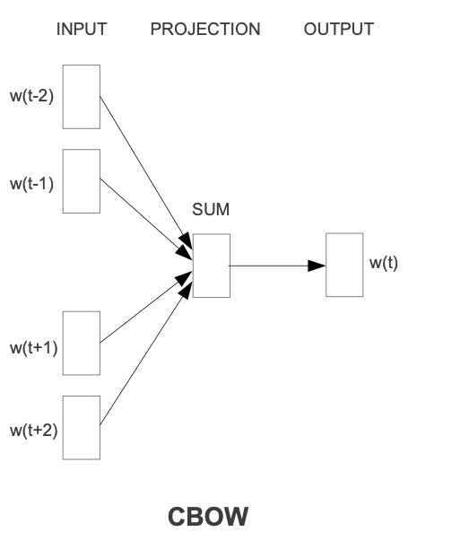
The CBOW model consists of three layers:
1. Input Layer:
Receives context words as one-hot vectors. Each word in the vocabulary is represented as a vector where only one element is 1 (indicating the word) and the rest are 0s.
Example: If “The” is the first word in a 10-word vocabulary, its one-hot representation would be
[1, 0, 0, 0, 0, 0].
2. Hidden Layer (Projection Layer):
This layer computes the average of the context words’ vectors, but there’s an important step before averaging.
Each one-hot vector is multiplied by a shared weight matrix to obtain a dense vector representation of each word. This matrix contains learned word features.
After converting each context word into its dense vector form, these vectors are averaged. This average represents the combined features of the context words.
Example: If “The” is transformed into a dense vector like [0.1, 0.2, 0.3, 0.4, 0.5, 0.6, 0.7, 0.8, 0.9, 1.0], and if it’s the only context word, this vector itself would be the output of the projection layer. If there are more context words, their transformed vectors are averaged with this.
3. Output Layer:
Predicts the current (target) word based on the combined context representation from the projection layer.
Uses a softmax function to output a probability distribution over the entire vocabulary. The word with the highest probability is chosen as the prediction.
Continuous Skip-gram
The Skip-gram model predicts the context based on the current word. For example, if we have the sentence “The cat is on the mat” and the context is 2, the model will predict the context “The cat __ on the mat” based on the word “is”.
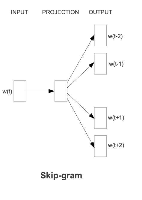
The Skip-gram model consists of three layers:
1. Input Layer:
Receives the current word represented as a one-hot vector.
Example: If “is” is the ninth word in a 10-word vocabulary, its one-hot representation would be [0, 0, 0, 0, 0, 0, 0, 0, 1, 0].
2. Hidden Layer (Projection Layer):
Similar to the CBOW model, the hidden layer in Skip-gram also uses a shared weight matrix. However, the process is somewhat reversed. In Skip-gram, the current word (represented as a one-hot vector) is used to predict the context words.
The one-hot vector is multiplied by the shared weight matrix to produce a dense vector representation of the current word. This matrix functions the same way as in CBOW, transforming sparse one-hot vectors into rich, dense word embeddings.
Example: The transformation of “is” might result in a dense vector like [0.1, 0.2, 0.3, 0.4, 0.5, 0.6, 0.7, 0.8, 0.9, 1.0].
3. Output Layer:
The output layer in Skip-gram is responsible for predicting the context words based on the dense vector representation of the current word.
Unlike CBOW, which uses the context to predict a single target word, Skip-gram uses the current word to predict multiple context words. This is typically achieved using multiple softmax classifiers, one for each context position.
Example: if the context window size is 2, there would be four softmax classifiers (two predicting the preceding words and two predicting the following words).
Semantic Similarity with Word2Vec
What makes Word2Vec so powerful is that the model can understand the semantics of the words and calculate the similarity between them. For example, if we have the following words:
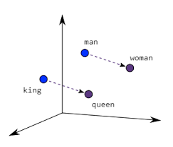
On this example we can see that Word2Vec can understand the semantics of the words and calculate the similarity between them. Also being represented as:
\[vector(king) - vector(man) + vector(woman) = vector(queen)\]The Word2Vec model is trained using a neural network which is responsible to learn the semantics of the words and represent them as vectors. With this approach we can calculate the similarity between words and documents.
Nowadays (2024) vector models still being used on a variety of tasks such as: document classification, document clustering, document retrieval, etc. But they have a problem, which is the curse of dimensionality. To solve this problem, Johnson et al. presented Annoy in 2017, which is a library that uses Approximate Nearest Neighbors to find the most similar documents based on a query.
Generating text with Seq2Seq Models (1980+)
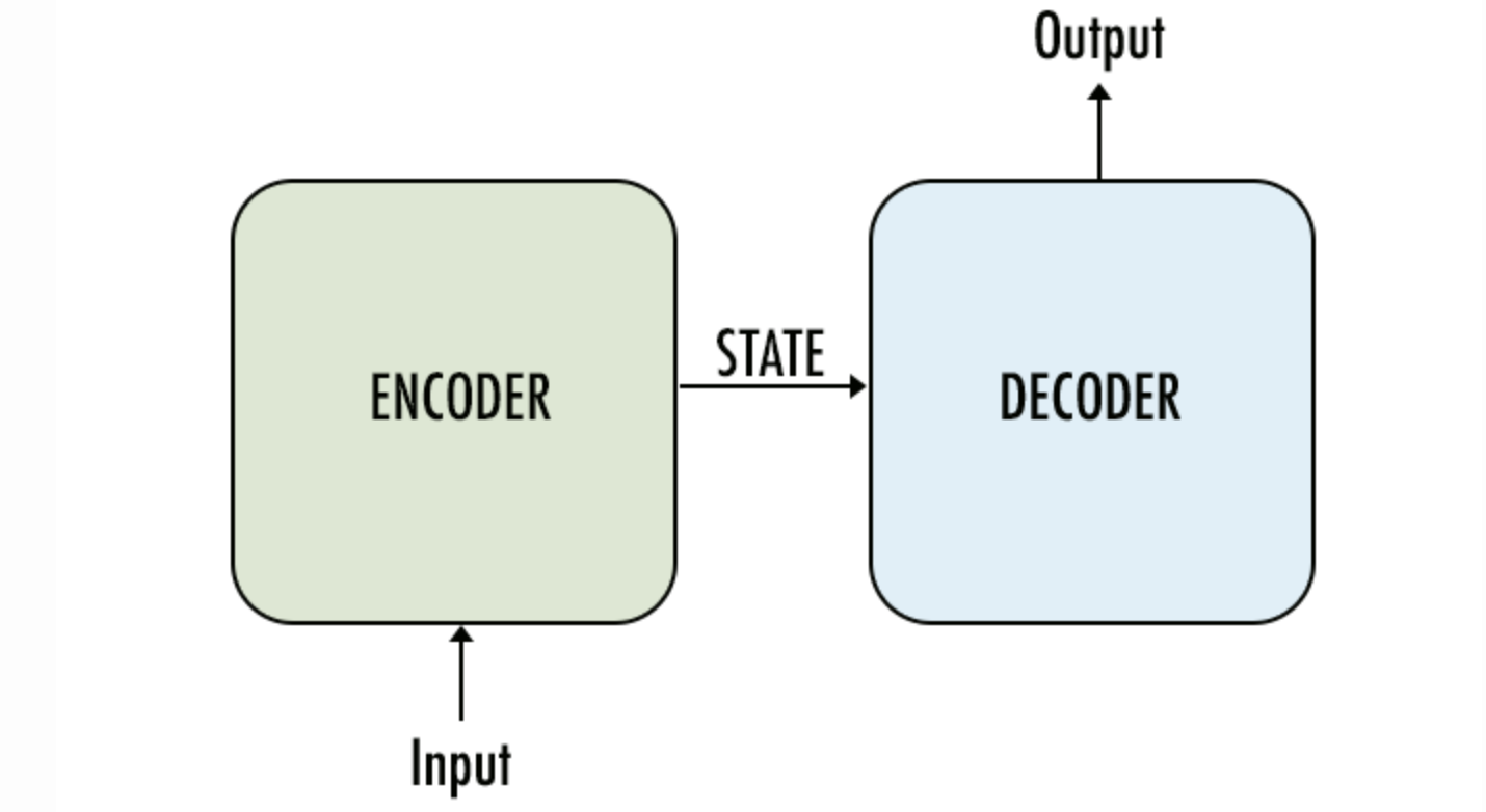
Seq2Seq Models also known as encoder-decoder models are a class of neural networks that are used to map sequences to sequences (e.g., text to text, audio to text, etc). It can be used in a variety of tasks such as: machine translation, text summarization, question answering, etc.
They are composed of two main components: an encoder and a decoder. The encoder is responsible to encode the input sequence into a numeric representation, and the decoder is responsible to decode the numeric representation into the output sequence.
Recurrent Neural Networks (RNNs):
RNNs for a long time were the most used approach to Seq2Seq Models. They are a class of neural networks that are used to process sequential data. They are composed of a hidden state that is passed to the next step of the sequence, allowing the model to learn the context of the sequence.
The problem with RNNs is that they have a short-term memory, which means that they can’t learn long sequences. To solve this problem, Hochreiter and Schmidhuber presented Long Short-Term Memory (LSTM) in 1997, which is a type of RNN that can learn long sequences.
But even with LSTM, RNNs still have a problem with long sequences, which is the vanishing gradient problem. To solve this problem, Cho et al. presented Gated Recurrent Unit (GRU) in 2014, which is a type of RNN that can learn long sequences without the vanishing gradient problem.
The problem with RNNs is that they are sequential, which means that they can’t be parallelized. To solve this problem, Vaswani et al. presented Transformer in 2017, which is a type of Seq2Seq Model that can learn long sequences and can be parallelized.
Attention Mechanism:
In 2017, Vaswani et al. presented Transformer, a new approach to Seq2Seq Models which is based on the attention mechanism. The attention mechanism is a technique that allows the model to focus on the most relevant parts of the input sequence to predict the next word.
The attention mechanism is composed of three main components: Query, Key, Value (QKV). It works similiar to a key-value database, where the query is used to retrieve the value of the most relevant key-value pairs. For example, if we have the following query:
query = "What is the capital of Brazil?"And the following key-value pairs:
key_value_pairs = [
  ("Brazil", "Brasilia"),
  ("France", "Paris"),
  ("Germany", "Berlin"),
  ("Italy", "Rome"),
  ("Japan", "Tokyo"),
  ("United States", "Washington, D.C.")
]
The attention mechanism will retrieve the most relevant key-value pairs based on the query. In this case, the most relevant key-value pair is ("Brazil", "Brasilia").
With this approach language models can learn the context of the sequence and generate more coherent text.
Pre-trained Language Models and The Role of Attention:
Pre-trained language models, a class of Seq2Seq Models, initially train on extensive text corpuses. Introduced in 2018 were BERT by Google AI and Generative Pre-trained Transformer (GPT) by OpenAI.
These models are trained on large corpuses of text, and they learn the semantics of the words and the context of the sequence. With this approach we can use these models to generate text, which is a task that was previously done by RNNs.
The problem is that these models doesn’t have access to external knowledge, which means that they can’t generate text based on your personal data or on up-to-date data without an expensive fine-tuning process or with accessing external knowledge during inference.
Synthesizing documents and generated text (2020)
Retrieval-augmented generation for Knowledge-Intensive NLP tasks was first introduced in 2020 in this paper where the author presented the defects of LLMs in accessing and manipulating external knowledge (e.g., your personal documents).
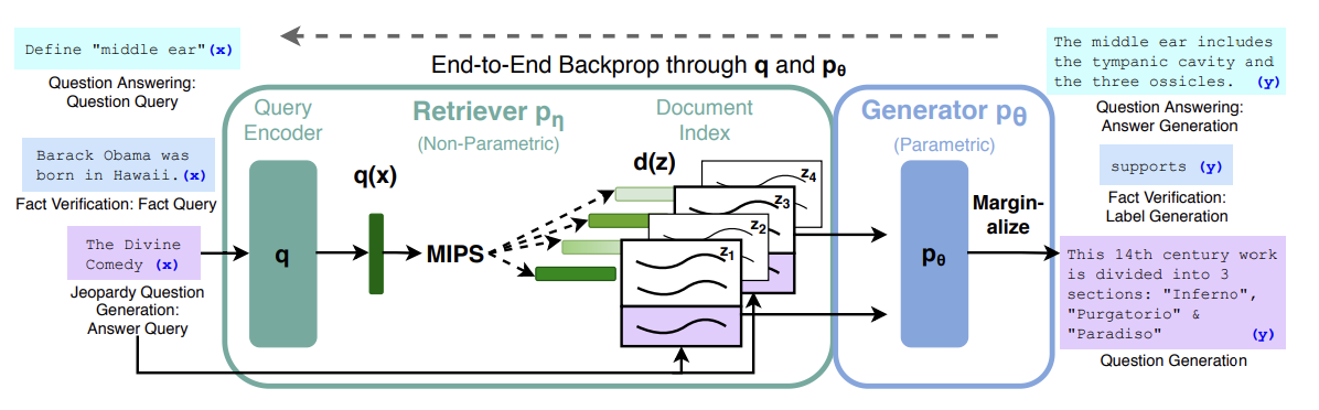
For RAG the author proposed a new architecture that combines a LLM with a retriever to access external knowledge being the retriever responsible to retrieve the most relevant documents based on a query and the LLM responsible to generate text based on the retrieved documents.
The architecture is composed of three main components: Query, Retriever, Generator. The query is the input of the system, which can be a text, image, audio, etc. The retriever is responsible to retrieve the most relevant documents based on the query. And the generator is responsible to synthesize the retrieved documents and generate the augmented answer.
Conclusion
Now we have a better understanding of the fundamentals of RAG, which is a combination of Information Retrieval (IR) and Seq2Seq Models. With this approach we can use our own data with Large Language Models (LLMs) (e.g., GPT-4, LLama2).
The RAG field is still emerging and there are a lot of failure points to be solved and challenges to be addressed. Companies like LlamaIndex have been working on this field and providing high-level and low-level APIs to use RAG in your applications on an easy way.
Wanna discuss about RAG? DM me on Twitter